Definition 3.5.1.
A basis \(\mathcal{B}\) is said to be an orthogonal basis if each pair of vectors in \(\mathcal{B}\text{,}\) \(\vec{\beta}_i\) and \(\vec{\beta}_j\text{,}\) are orthogonal 1 . If in addition \(||\vec{\beta}_i||=1\) for all \(i\) then we say that the basis is orthonormal.
Investigation 3.5.1. Orthogonal and Non-Orthogonal Bases.
Consider the bases
\begin{equation*}
\mathcal{B}=
\left\{
\left[
\begin{array}{r}
2 \\ 0 \\ 1
\end{array}
\right],
\left[
\begin{array}{r}
0 \\ 1 \\ 0
\end{array}
\right],
\left[
\begin{array}{r}
-1 \\ 0 \\ 2
\end{array}
\right]
\right\}
\end{equation*}
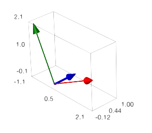
Figure 3.5.2. Orthogonal Basis
and
\begin{equation*}
\mathcal{D}=
\left\{
\left[
\begin{array}{r}
1 \\ 1 \\ 1
\end{array}
\right],
\left[
\begin{array}{r}
0 \\ 1 \\ 1
\end{array}
\right],
\left[
\begin{array}{r}
0 \\ 0 \\ 1
\end{array}
\right]
\right\}.
\end{equation*}
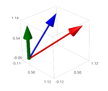
Figure 3.5.3. Non-Orthogonal Basis
Both of the above sets are bases for \(\mathbb{R}^3\) but only \(\mathcal{B}\) is an orthogonal basis. We can see this because
\begin{align*}
\left\lt2,0,1\right\gt\cdot\left\lt0,1,0\right\gt\amp=0\\
\left\lt2,0,1\right\gt\cdot\left\lt-1,0,2\right\gt\amp=0,\ \mbox{ and}\\
\left\lt-1,0,2\right\gt\cdot\left\lt0,1,0\right\gt\amp=0.
\end{align*}
However, \(\mathcal{D}\) is not since
\begin{equation*}
\left\lt1,1,1\right\gt\cdot\left\lt0,1,1\right\gt=2,
\end{equation*}
so there is at least one pair of vectors which are not orthogonal.
Further if we replace \(\mathcal{B}\) with
\begin{equation*}
\mathcal{B'}=
\left\{
\left[
\begin{array}{r}
\frac{2}{\sqrt{3}} \\ 0 \\ \frac{1}{\sqrt{3}}
\end{array}
\right],
\left[
\begin{array}{r}
0 \\ 1 \\ 0
\end{array}
\right],
\left[
\begin{array}{r}
-\frac{1}{\sqrt{3}} \\ 0 \\ \frac{2}{\sqrt{3}}
\end{array}
\right]
\right\}
\end{equation*}
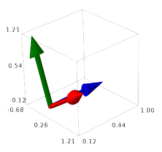
Figure 3.5.4. Orthonormal Basis
we have an orthonormal basis since all the vectors now have length one and are perpendicular. Moreover, since all of these vectors point in the same direction as the vectors of \(\mathcal{B}\) we can call this the normalization of \(\mathcal{B}\text{.}\)
Investigation 3.5.2. Orthogonalization.
Consider again
\begin{equation*}
\mathcal{D}=
\left\{
\left[
\begin{array}{r}
1 \\ 1 \\ 1
\end{array}
\right],
\left[
\begin{array}{r}
0 \\ 1 \\ 1
\end{array}
\right],
\left[
\begin{array}{r}
0 \\ 0 \\ 1
\end{array}
\right]
\right\}.
\end{equation*}
and suppose that we want to develop an orthonormal basis from this. We will do this a step at a time using the Gram-Schmidt Orthogonalization process.
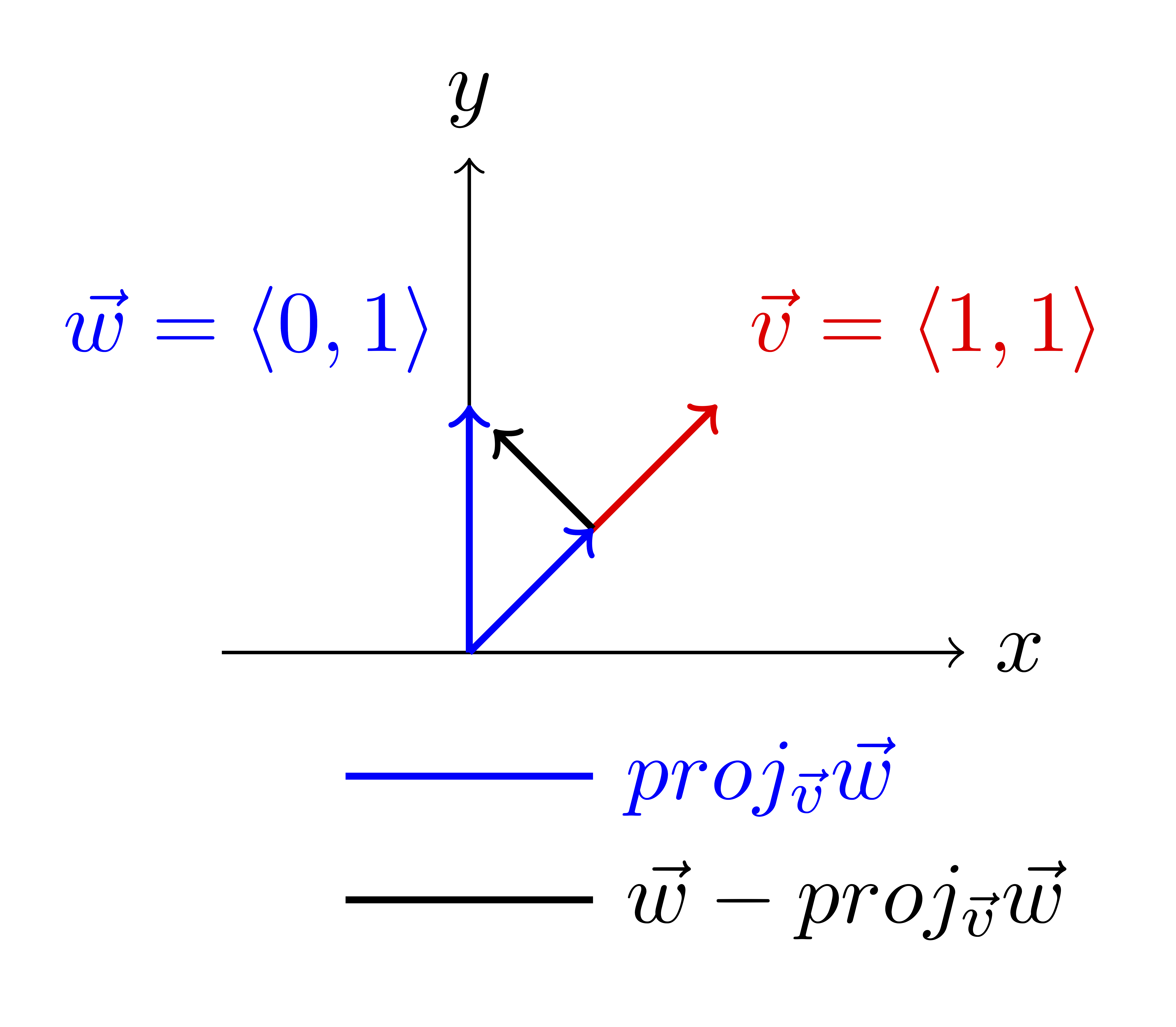
The process is based on the vector projections we studied before. If \(\vec{v}=\left\lt1,1\right\gt\) and \(\vec{w}=\left\lt0,1\right\gt\text{,}\) then
\begin{equation*}
proj_{\vec{v}}\vec{w}=\frac{\vec{v}\cdot\vec{w}}{\vec{v}\cdot\vec{v}}\vec{v}=\left\lt\frac{1}{2},\frac{1}{2}\right\gt.
\end{equation*}
The vector
\begin{equation*}
\vec{w}-proj_{\vec{v}}\vec{w}=\left\lt-\frac{1}{2},\frac{1}{2}\right\gt.
\end{equation*}
is an orthogonal complement of the projection; it is orthogonal to \(\vec{v}\) and we can use it to replace \(\vec{w}\text{.}\)
Figure 3.5.5.
Consider
\begin{align*}
a\vec{v}+b\vec{w}\amp = a\vec{v}+b\vec{w}\\
\amp = a\vec{v}+b\, \left(\vec{w}-proj_{\vec{v}}\vec{w}+proj_{\vec{v}}\vec{w}\right)\\
\amp = a\vec{v}+b\, proj_{\vec{v}}\vec{w}+b\, \left(\vec{w}-proj_{\vec{v}}\vec{w}\right)\\
\amp = a\vec{v}+\frac{b}{2}\vec{v}+b\, \left(\vec{w}-proj_{\vec{v}}\vec{w}\right),\\
\amp = \left(a+\frac{b}{2}\right)\vec{v}+b\, \left(\vec{w}-proj_{\vec{v}}\vec{w}\right),
\end{align*}
so we can systematically replace any linear combination of \(\vec{v}\) and \(\vec{w}\) with a combination of \(\vec{v}\) and \(\vec{w}-proj_{\vec{v}}\vec{w}\text{.}\) This is the Gram-Schmidt Orthogonalization process.