
Section 3.2 Matrix Operations

Subsection 3.2.1 Basic Matrix Arithmetic

Investigation 3.2.1. Addition.

Matrix addition is done term by term.

\begin{align*} \left( \begin{array}{rrr} 2\amp 0 \amp 5\\ -1\amp 3 \amp 4 \end{array} \right)+ \left( \begin{array}{rrr} 0\amp 5 \amp 1\\ 1\amp 7 \amp -2 \end{array} \right)\amp = \left( \begin{array}{rrr} 2+0\amp 0+5 \amp 5+1\\ -1+1\amp 3+7 \amp 4+(-2) \end{array} \right)\\ \amp = \left( \begin{array}{rrr} 2\amp 5 \amp 6\\ 0\amp 10 \amp 2 \end{array} \right) \end{align*}
Investigation 3.2.2. Scalar Multiplication.

Scalar multiplication is likewise done term by term.

\begin{align*} 5 \left( \begin{array}{rrr} 2\amp 0 \amp 5\\ -1\amp 3 \amp 4 \end{array} \right)\amp = \left( \begin{array}{rrr} 5(2)\amp 5(0) \amp 5(5)\\ 5(-1)\amp 5(3) \amp 5(4) \end{array} \right)\\ \amp = \left( \begin{array}{rrr} 10\amp 0 \amp 25\\ -5\amp 15 \amp 20 \end{array} \right) \end{align*}
Investigation 3.2.3. Matrix Multiplication.

Multiply the rows of the first matrix by the columns of the second, multiplication is taking the dot product of rows with columns.

\begin{align*} \left( \begin{array}{rrr} 2\amp 0 \amp 5\\ -1\amp 3 \amp 4 \end{array} \right) \left( \begin{array}{rr} 0\amp 5 \\ 1\amp 7 \\ 0\amp 1 \end{array} \right)\amp = \left( \begin{array}{rr} 2(0)+0(1)+5(0) \amp 2(5)+0(7)+5(1) \\ -1(0)+3(1)+4(0) \amp -1(5)+3(7)+4(1) \end{array} \right)\\ \amp = \left( \begin{array}{rr} 0\amp 15 \\ 3\amp 20 \end{array} \right) \end{align*}
Investigation 3.2.4. Putting it All Together:.
\begin{align*} 2 \left( \begin{array}{rr} 1\amp -7 \\ 3\amp 2 \end{array} \right)+ \left( \begin{array}{rrr} 2\amp 0 \amp 5\\ -1\amp 3 \amp 4 \end{array} \right) \left( \begin{array}{rr} 0\amp 5 \\ 1\amp 7 \\ 0\amp 1 \end{array} \right)\amp = \left( \begin{array}{rr} 2(1)\amp 2(-7) \\ 2(3)\amp 2(2) \end{array} \right)+ \left( \begin{array}{rr} 2(0)+0(1)+5(0) \amp 2(5)+0(7)+5(1) \\ -1(0)+3(1)+4(0) \amp -1(5)+3(7)+4(1) \end{array} \right)\\ \amp = \left( \begin{array}{rr} 2\amp -14 \\ 6\amp 4 \end{array} \right)+ \left( \begin{array}{rr} 0 \amp 15 \\ 3 \amp 20 \end{array} \right)\\ \amp = \left( \begin{array}{rr} 2+0 \amp -14+15 \\ 6+3 \amp 4+20 \end{array} \right)\\ \amp = \left( \begin{array}{rr} 2 \amp 1 \\ 9 \amp 24 \end{array} \right) \end{align*}

Subsection 3.2.2 Invertible Matrices

Definition 3.2.1.

A matrix \(A\) is invertible is there exists a matrix \(A^{-1}\) such that \(A\, A^{-1}=A^{-1}\, A=I\) where \(I\) is the identity matrix. If there exists \(B\) such that only \(A\, B=I\) and \(B\, A\neq I\text{,}\) then \(B\) is the right inverse of \(A\) and \(A\) is the left inverse of \(B\text{.}\)

Investigation 3.2.5. \(2\times 2\) - Matrix Version 1.

Find the inverse of

\begin{equation*} A=\left( \begin{array}{rr} 2 \amp 5 \\ 3 \amp 8 \end{array} \right). \end{equation*}

We want to find

\begin{equation*} A^{-1}=\left( \begin{array}{rr} a \amp b \\ c \amp d \end{array} \right) \end{equation*}

so that

\begin{equation*} A\, A^{-1}= \left( \begin{array}{rr} 2 \amp 5 \\ 3 \amp 8 \end{array} \right) \left( \begin{array}{rr} a \amp b \\ c \amp d \end{array} \right)= \left( \begin{array}{rr} 1 \amp 0 \\ 0 \amp 1 \end{array} \right). \end{equation*}

Multiplyting as above this reduces to

\begin{equation*} \left( \begin{array}{rr} 2a+5c \amp 2b+5d \\ 3a+8c \amp 3b+8d \end{array} \right)= \left( \begin{array}{rr} 1 \amp 0 \\ 0 \amp 1 \end{array} \right) \end{equation*}

or

\begin{gather*} 2a+5c=1\\ 3a+8c=0 \end{gather*}

and

\begin{gather*} 2b+5d=0\\ 3b+8d=1. \end{gather*}

We get two sets of two equations each with two variables. Writing each of these as augmented matrices we get

\begin{equation*} \left( \begin{array}{rr|r} 2 \amp 5 \amp 1\\ 3 \amp 8 \amp 0 \end{array} \right) \end{equation*}

and

\begin{equation*} \left( \begin{array}{rr|r} 2 \amp 5 \amp 0\\ 3 \amp 8 \amp 1 \end{array} \right). \end{equation*}

Solving each of these we would get \(a=8\text{,}\) \(b=-5\text{,}\) \(c=-3\text{,}\) and \(d=2\text{,}\) so

\begin{equation*} A^{-1}=\left( \begin{array}{rr} 8 \amp -5 \\ -3 \amp 2 \end{array} \right). \end{equation*}

But, notice that the coefficient matrices are the same for both systems of equations, they are both \(A\text{,}\) so that when we reduce them we follow the same steps each time, this gives us a better way to approach this.

Investigation 3.2.6. \(2\times 2\) - Matrix Version 2.

Find the inverse of

\begin{equation*} A=\left( \begin{array}{rr} 2 \amp 5 \\ 3 \amp 8 \end{array} \right). \end{equation*}

We want to find

\begin{equation*} A^{-1}=\left( \begin{array}{rr} a \amp b \\ c \amp d \end{array} \right) \end{equation*}

so that

\begin{equation*} A\, A^{-1}= \left( \begin{array}{rr} 2 \amp 5 \\ 3 \amp 8 \end{array} \right) \left( \begin{array}{rr} a \amp b \\ c \amp d \end{array} \right)= \left( \begin{array}{rr} 1 \amp 0 \\ 0 \amp 1 \end{array} \right). \end{equation*}

From above we want a coefficient matrix that matches \(A\) and then two vectors on the right which together match the identity matrix, so it looks like this

\begin{equation*} \left( \begin{array}{rr|rr} 2 \amp 5 \amp 1\amp 0\\ 3 \amp 8 \amp 0 \amp 1 \end{array} \right). \end{equation*}

Let's see what we get when we row reduce the left hand side:

\begin{align*} \left( \begin{array}{rr|rr} 2 \amp 5 \amp 1\amp 0\\ 3 \amp 8 \amp 0 \amp 1 \end{array} \right)\amp \leadsto \left( \begin{array}{rr|rr} 3 \amp 8 \amp 0\amp 1\\ 2 \amp 5 \amp 1 \amp 0 \end{array} \right)\\ \amp \leadsto \left( \begin{array}{rr|rr} 3 \amp 8 \amp 0\amp 1\\ 2 \amp 5 \amp 1 \amp 0 \end{array} \right)\\ \amp \leadsto \left( \begin{array}{rr|rr} 1 \amp 3 \amp -1\amp 1\\ 2 \amp 5 \amp 1 \amp 0 \end{array} \right)\\ \amp \leadsto \left( \begin{array}{rr|rr} 1 \amp 3 \amp -1\amp 1\\ 0 \amp -1 \amp 3 \amp -2 \end{array} \right)\\ \amp \leadsto \left( \begin{array}{rr|rr} 1 \amp 3 \amp -1\amp 1\\ 0 \amp 1 \amp -3 \amp 2 \end{array} \right)\\ \amp \leadsto \left( \begin{array}{rr|rr} 1 \amp 0 \amp 8\amp -5\\ 0 \amp 1 \amp -3 \amp 2 \end{array} \right). \end{align*}

What we got on the right is exactly the inverse we wanted

\begin{equation*} A^{-1}=\left( \begin{array}{rr} 8 \amp -5 \\ -3 \amp 2 \end{array} \right). \end{equation*}

This is really the same thing we did before, but we did it all at once to save time.

As a final note on \(2\times 2\) matrices if

\begin{equation*} A=\left( \begin{array}{rr} a \amp b \\ c \amp d \end{array} \right) \end{equation*}

then it turns out

\begin{equation*} A^{-1}=\frac{1}{ad-bc}\left( \begin{array}{rr} d \amp -b \\ -c \amp a \end{array} \right) \end{equation*}

provided \(ad-bc\neq 0\text{;}\) if \(ad-bc=0\) then \(A\) doesn't have an inverse. Unfortunately, there is not such a simple formula for larger matrices.

Investigation 3.2.7. Inverse of a \(3\times 3\) Matrix.

Find the inverse of

\begin{equation*} A=\left( \begin{array}{rrr} 1 \amp 0 \amp -1 \\ 3 \amp 8 \amp 0 \\ 0 \amp 4 \amp 2 \\ \end{array} \right). \end{equation*}

As before we set up an augmented matrix with \(A\) as the coefficients on the left and vectors on the right that when taken together look like the identity matrix, then we row reduce.

\begin{align*} \left( \begin{array}{rrr|rrr} 1 \amp 0 \amp -1 \amp 1 \amp 0 \amp 0 \\ 3 \amp 8 \amp 0 \amp 0 \amp 1 \amp 0 \\ 0 \amp 4 \amp 2 \amp 0 \amp 0 \amp 1\\ \end{array} \right) \amp\leadsto \left( \begin{array}{rrr|rrr} 1 \amp 0 \amp -1 \amp 1 \amp 0 \amp 0 \\ 0 \amp 8 \amp 3 \amp -3 \amp 1 \amp 0 \\ 0 \amp 8 \amp 4 \amp 0 \amp 0 \amp 2\\ \end{array} \right)\\ \amp\leadsto \left( \begin{array}{rrr|rrr} 1 \amp 0 \amp -1 \amp 1 \amp 0 \amp 0 \\ 0 \amp 8 \amp 3 \amp -3 \amp 1 \amp 0 \\ 0 \amp 0 \amp 1 \amp 3 \amp -1 \amp 2\\ \end{array} \right)\\ \amp\leadsto \left( \begin{array}{rrr|rrr} 1 \amp 0 \amp 0 \amp 4 \amp -1 \amp 2 \\ 0 \amp 8 \amp 0 \amp -12 \amp 4 \amp -6 \\ 0 \amp 0 \amp 1 \amp 3 \amp -1 \amp 2\\ \end{array} \right)\\ \amp\leadsto \left( \begin{array}{rrr|rrr} 1 \amp 0 \amp 0 \amp 4 \amp -1 \amp 2 \\ 0 \amp 1 \amp 0 \amp -\frac{3}{2} \amp \frac{1}{2} \amp -\frac{3}{4} \\ 0 \amp 0 \amp 1 \amp 3 \amp -1 \amp 2\\ \end{array} \right) \end{align*}

So that we get

\begin{equation*} A^{-1}= \left( \begin{array}{rrr} 4 \amp -1 \amp 2 \\ -\frac{3}{2} \amp \frac{1}{2} \amp -\frac{3}{4} \\ 3 \amp -1 \amp 2\\ \end{array} \right). \end{equation*}
Investigation 3.2.8. Inverse of a \(4\times 4\) Matrix.

Find the inverse of

\begin{equation*} A=\left( \begin{array}{rrrr} 1 \amp 0 \amp 1 \amp 5 \\ 3 \amp 1 \amp 0 \amp 15\\ 0 \amp 1 \amp -2 \amp 0\\ 7 \amp 5 \amp 8 \amp 36 \end{array} \right). \end{equation*}

As before we set up an augmented matrix with \(A\) as the coefficients on the left and vectors on the right that when taken together look like the identity matrix, then we row reduce.

\begin{align*} \left( \begin{array}{rrrr|rrrr} 1 \amp 0 \amp 1 \amp 5 \amp 1 \amp 0 \amp 0 \amp 0\\ 3 \amp 1 \amp 0 \amp 15 \amp 0 \amp 1 \amp 0 \amp 0\\ 0 \amp 1 \amp -2 \amp 0 \amp 0 \amp 0 \amp 1 \amp 0\\ 2 \amp 3 \amp -7 \amp 11 \amp 0 \amp 0 \amp 0 \amp 1 \end{array} \right) \amp\leadsto \left( \begin{array}{rrrr|rrrr} 1 \amp 0 \amp 1 \amp 5 \amp 1 \amp 0 \amp 0 \amp 0\\ 0 \amp 1 \amp -3 \amp 0 \amp -3 \amp 1 \amp 0 \amp 0\\ 0 \amp 1 \amp -2 \amp 0 \amp 0 \amp 0 \amp 1 \amp 0\\ 0 \amp 3 \amp -9 \amp 1 \amp -2 \amp 0 \amp 0 \amp 1 \end{array} \right)\\ \amp\leadsto \left( \begin{array}{rrrr|rrrr} 1 \amp 0 \amp 1 \amp 5 \amp 1 \amp 0 \amp 0 \amp 0\\ 0 \amp 1 \amp -3 \amp 0 \amp -3 \amp 1 \amp 0 \amp 0\\ 0 \amp 0 \amp 1 \amp 0 \amp 3 \amp -1 \amp 1 \amp 0\\ 0 \amp 0 \amp 0 \amp 1 \amp 7 \amp -3 \amp 0 \amp 1 \end{array} \right)\\ \amp\leadsto \left( \begin{array}{rrrr|rrrr} 1 \amp 0 \amp 0 \amp 0 \amp -37 \amp 16 \amp -1 \amp -5\\ 0 \amp 1 \amp 0 \amp 0 \amp 6 \amp -2 \amp 3 \amp 0\\ 0 \amp 0 \amp 1 \amp 0 \amp 3 \amp -1 \amp 1 \amp 0\\ 0 \amp 0 \amp 0 \amp 1 \amp 7 \amp -3 \amp 0 \amp 1 \end{array} \right) \end{align*}

So that we get

\begin{equation*} A^{-1}= \left( \begin{array}{rrrr} -37 \amp 16 \amp -1 \amp -5\\ 6 \amp -2 \amp 3 \amp 0\\ 3 \amp -1 \amp 1 \amp 0\\ 7 \amp -3 \amp 0 \amp 1 \end{array} \right). \end{equation*}
Investigation 3.2.9. A Couple Non-Examples.

Suppose that we were given

\begin{equation*} A=\left( \begin{array}{rr} 2 \amp 3 \\ 4 \amp 6\\ \end{array} \right) \end{equation*}

and we were asked to find the inverse, could we do it? From what we mentioned above (Paragraph ) we know the answer is no because \(2(6)-3(4)=0\text{.}\) But, what woudl happen if we ignored this and tried any ways:

\begin{equation*} \left( \begin{array}{rr|rr} 2 \amp 3 \amp 1 \amp 0\\ 4 \amp 6 \amp 0 \amp 1\\ \end{array} \right) \leadsto \left( \begin{array}{rr|rr} 2 \amp 3 \amp 1 \amp 0\\ 0 \amp 0 \amp -2 \amp 1\\ \end{array} \right), \end{equation*}

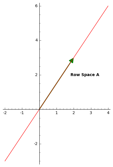
which is an inconsistent system. This happens because the row space of \(A\) is one dimensional, it is a single line in the direction of \(\left(2,3\right)\text{,}\) but it exists in two dimensions.

Figure 3.2.2. One Dimensional Row Space for a \(2\times 2\) matrix

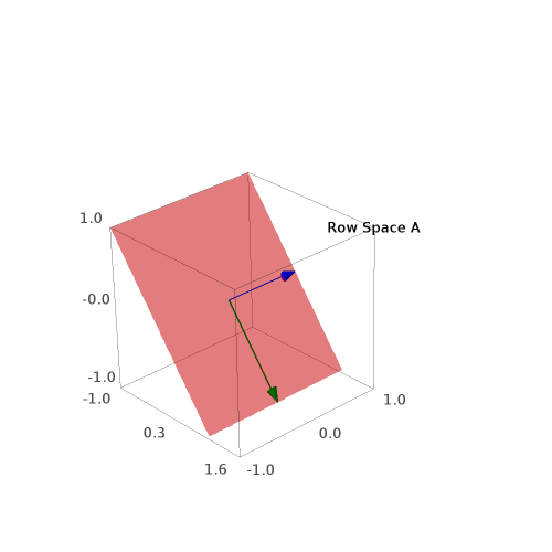
Now for a larger example, if we try to get an inverse for

\begin{equation*} A=\left( \begin{array}{rrr} 1 \amp 0 \amp -1\\ 0 \amp 1 \amp 0\\ 0 \amp 1 \amp 0\\ \end{array} \right) \end{equation*}

we get

\begin{equation*} \left( \begin{array}{rrr|rrr} 1 \amp 0 \amp -1 \amp 1 \amp 0 \amp 0\\ 0 \amp 1 \amp 0 \amp 0 \amp 1 \amp 0\\ 0 \amp 1 \amp 0 \amp 0 \amp 0 \amp 1\\ \end{array} \right) \leadsto \left( \begin{array}{rrr|rrr} 1 \amp 0 \amp -1 \amp 1 \amp 0 \amp 0\\ 0 \amp 1 \amp 0 \amp 0 \amp 1 \amp 0\\ 0 \amp 0 \amp 0 \amp 0 \amp -1 \amp 1\\ \end{array} \right). \end{equation*}

We can't row reduce \(A\) so we don't get an inverse. This is happening because the rows of \(A\) are not linearly independent, the row space for \(A\) is

\begin{align*} Row\ A\amp=\left\{\left( 1,0,-1\right), \left( 0,1,0\right) \right\} \end{align*}

which is only two dimensional. That is, a matrix which in a sense has a two dimensional span but exists in three dimensions doesn't have an inverse.

Figure 3.2.3. Two Dimensional Row Space for a \(3\times 3\) matrix

Note that while \(A\) doesn't have an inverse

\begin{equation*} \left( \begin{array}{rrr} 1 \amp 0 \amp -1\\ 0 \amp 1 \amp 0\\ \end{array} \right) \left( \begin{array}{rr} 1 \amp 0 \\ 0 \amp 1 \\ 0 \amp 0 \\ \end{array} \right)= \left( \begin{array}{rr} 1 \amp 0 \\ 0 \amp 1 \\ \end{array} \right), \end{equation*}
so that a matrix with the same row space has a right inverse. 1 You should convince yourself that it doesn't have a left inverse.
Concluding Remarks.

Using row reduction to get inverses is the standard introductory way to find them. It does take patience and precision, both of which can be bad at. Computers can do this very well though. Use the code below to help you check your work while practicing. You should also learn to use the computer to help you check your other calculations. (Make use of the Linear Algebra Quick Reference and you can use the box below or go to the SageMathCell main page.)