
Section 3.3 Linear Maps and Matrices

Subsection 3.3.1 Matrices as Maps

Investigation 3.3.1.

Let

\begin{equation*} A= \left( \begin{array}{rr} 1 \amp 0 \\ -3 \amp 1 \end{array} \right),\ \vec{w}= \left( \begin{array}{rr} 5\\ 1 \end{array} \right),\ \mbox{ and } \vec{v}= \left( \begin{array}{rr} -1\\ 10 \end{array} \right).\ \end{equation*}

We can "quickly" verify that \(A(2\vec{v}+\vec{w})=2(A\vec{v})+A\vec{w}\text{:}\)

\begin{align*} \left( \begin{array}{rr} 1 \amp 0 \\ -3 \amp 1 \end{array} \right) \left( 2\left( \begin{array}{rr} -1\\ 10 \end{array} \right)+ \left( \begin{array}{rr} 5\\ 1 \end{array} \right) \right)\amp= \left( \begin{array}{rr} 1 \amp 0 \\ -3 \amp 1 \end{array} \right) \left( \begin{array}{rr} -2+5\\ 20+1 \end{array} \right)\\ \amp= \left( \begin{array}{rr} 1(-2+5)+0(20+1)\\ -3(-2+5)+1(20+1)\\ \end{array} \right)\\ \amp= \left( \begin{array}{rr} 1(-2)+0(20)\\ -3(-2)+1(20)\\ \end{array} \right)+ \left( \begin{array}{rr} 1(5)+0(1)\\ -3(5)+1(1)\\ \end{array} \right)\\ \amp= 2\left( \begin{array}{rr} 1(-1)+0(10)\\ -3(-1)+1(10)\\ \end{array} \right)+ \left( \begin{array}{rr} 1 \amp 0 \\ -3 \amp 1 \end{array} \right) \left( \begin{array}{rr} 5\\ 1\\ \end{array} \right)\\ \amp= 2\left( \left( \begin{array}{rr} 1 \amp 0 \\ -3 \amp 1 \end{array} \right) \left( \begin{array}{rr} -1\\ 10\\ \end{array} \right) \right)+ \left( \begin{array}{rr} 1 \amp 0 \\ -3 \amp 1 \end{array} \right) \left( \begin{array}{rr} 5\\ 1\\ \end{array} \right) \end{align*}

What is true, though perhaps not immediately obvious, is that this doesn't depend on the values of \(A\text{,}\) \(\vec{w}\text{,}\) or \(\vec{v}\text{.}\)

Investigation 3.3.2.

The previous relationship works both ways. Define \(T:\mathbb{R}^3\rightarrow\mathbb{R}^2\) by

\begin{equation*} T(\left\lt x_1,x_2,x_3\right\gt)=\left\lt x_1-2x_2, 2x_2-3x_3\right\gt. \end{equation*}

If we apply this to each element of the elementary basis \(\mathcal{E}_3\) for \(\mathbb{R}^3\) we get:

\begin{align*} T(\left\lt 1,0,0\right\gt)\amp=\left\lt 1, 0\right\gt,\\ T(\left\lt 0,1,0\right\gt)\amp=\left\lt -2, 2\right\gt,\ \mbox{ and }\\ T(\left\lt 0,0,1\right\gt)\amp=\left\lt 0, -3\right\gt. \end{align*}

But, this is the same as multiplying each of the vectors by the matrix

\begin{equation*} \left( \begin{array}{rrr} 1 \amp -2 \amp 0\\ 0 \amp 2 \amp -3 \end{array} \right) \end{equation*}

in which each column is the image of one of the elementary vectors.

Subsection 3.3.2 Row, Column, and Null Spaces (again)

The row, column, and null spaces for the matrix

\begin{equation*} A=\left[ \begin{array}{rrr} 1 \amp 0 \amp -1\\ 0 \amp 1 \amp 0\\ 0 \amp 1 \amp 0\\ \end{array} \right] \end{equation*}

are

\begin{align*} Row\ A\amp=\left\{\left\lt 1,0,-1\right\gt, \left\lt 0,1,0\right\gt \right\}, \\ Col\ A\amp=\left\{\left\lt 1,0,0\right\gt, \left\lt 0,1,1\right\gt \right\}, and\\ Nul\ A\amp=\left\{\left\lt 1,0,1\right\gt\right\}. \end{align*}

We can see these visually in Figure 3.3.3 where you can see the plain of the row space transition to the plain of the column space while the vector of the null space transitions to zero.

Figure 3.3.3. Row and Null Spaces Transitioning to Column Space and Zero

If we multiply each of the standard basis elements by the matrix \(A\) we get

\begin{gather*} \vec{e}_1=\left\lt 1,0,0 \right\gt \leadsto \left\lt 1,0,0 \right\gt\\ \vec{e}_2=\left\lt 0,1,0 \right\gt \leadsto \left\lt 0,1,1 \right\gt\\ \vec{e}_3=\left\lt 0,0,1 \right\gt \leadsto \left\lt -1,0,0 \right\gt \end{gather*}

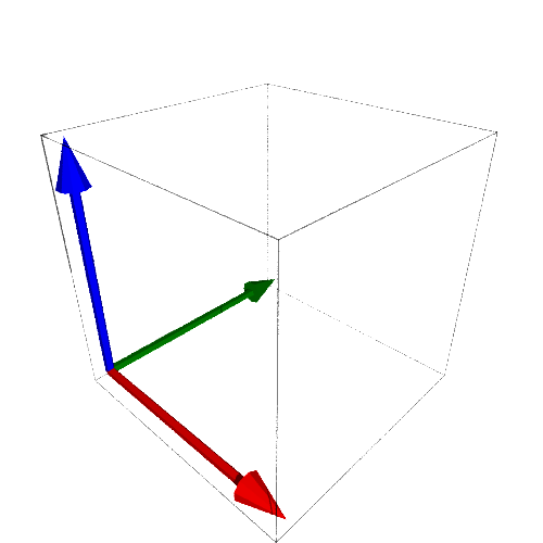
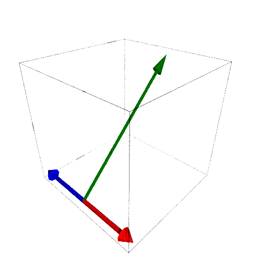
which are the columns of the matrix. The domain of the transformation defined by \(A\) is therefore \(\mathbb{R}^3\text{,}\) Figure 3.3.4. Meanwhile, the image (or range) of the transformation is the column space of \(A\) which is a copy of \(\mathbb{R}^2\text{,}\) Figure 3.3.5. So the basis for \(\mathbb{R}^3\) has been turned into a basis for a plain that is a copy of \(\mathbb{R}^2\text{.}\) 1 This is the perspective that we will spend time on in Section 3.4.

Figure 3.3.4. Standard Basis Before Transformation
Figure 3.3.5. Basis After Transformation by \(A\)

We can also define a linear transformation \(T_A\) algebraically by

\begin{equation*} \left( \begin{array}{c} x\\ y \\ z \end{array} \right) \stackrel{T_A}{\leadsto} \left( \begin{array}{c} x-z\\ y \\ y \end{array} \right) \end{equation*}

which has the same effect as multiplying the vector \(\left\lt x,y,z\right\gt\) by \(A\text{.}\)

We have three ways to think of each transformation. Each transformation is a manipulation of a physical space, a change from one basis to another, or a series of algebraic instructions. All of these are reasonable ways to view a transformation and which perspective we use depends on what we wish to accomplish.