Section 3.1 Isomorphisms and Homomorphisms of Vector Spaces
¶Subsection 3.1.1 Homorphisms and Functions
Definition 3.1.1.
A function is a relation, call it \(A\text{,}\) from one set called the domain, \(X\text{,}\) to another set called the codomain, \(Y\) such that
- \(\forall x\in X,\ \exists y\in Y:\ A(x)=y\)
- \(\forall x\in X:\) if \(y_1=A(x)\) and \(y_2=A(x)\text{,}\) then \(y_1=y_2\text{.}\)
If in addition we know that \(A(ax+by)=a\, A(x)\, +\, b\, A(y)\) we say that the function is a homomorphism, or that it is a linear map.
Investigation 3.1.1. Something Linear.
Let \(f:\mathbb{R}\rightarrow\mathbb{R}\) be defined by \(f(x)=-7x\) and let's see that this is linear. First, since both the input and output for the function comes from \(\mathbb{R}\) that is the domain and the codomain. If \(x=ax_1+bx_2\text{,}\) then we get
Therefore, \(f(x)\) satisfies the definition of a homomorphism (linear function).
Investigation 3.1.2. Also Linear.
Let \(d:\mathcal{P}_3\rightarrow\mathcal{P}_3\) be defined by \(d(f)=3ax^2+2bx+c\) and let's see that this too is linear. First, since both the input and output for the function comes from \(\mathcal{P}_3\) that is the domain and the codomain. If \(f(x)=a_1x^3+b_1x^2+c_1x+d_1\) and \(g(x)=a_2x^3+b_2x^2+c_2x+d_2\text{,}\) then we get
and when we apply the function \(d\)
Therefore, \(d\) satisfies the definition of a homomorphism (linear function).
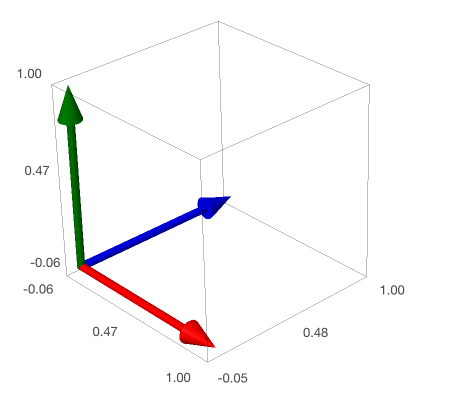
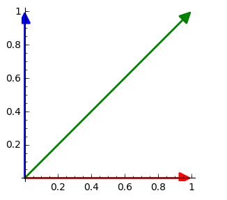
Investigation 3.1.3. Something with Vectors.
Define \(T:\mathbb{R}^3\rightarrow\mathbb{R}^2\) by
For example:
This is a linear map since
Investigation 3.1.4. Surprisingly Not Linear.
Let \(f:\mathbb{R}\rightarrow\mathbb{R}\) be defined by \(f(x)=x+1\) and let's see that this is not linear. Since we want to see that something is not the case we just need a counter example. If \(x=1\) and \(y=2\) then
but
so that \(f(x)+f(y)\neq f(x+y)\text{,}\) i.e. \(f\) is not linear. This may be surprising since \(f(x)=x+1\) is a line, but this is what is called an affine map since it is the sum of a linear map and a constant.
Subsection 3.1.2 Isomorphisms (one-to-one and onto)
Definition 3.1.4.
A function \(f:V\rightarrow W\) is one-to-one if for all \(v_1,v_2\in V\text{,}\) \(f(v_1)=f(v_2)\) implies \(v_1=v_2\text{.}\) The function is onto if for all \(w\in W\) there exists \(v\in V\) such that \(f(v)=w\text{.}\) A function which is both is called an isomorphism.
Looking back at Investigation 3.1.1 the function is an isomorphism. If \(-7x_1=-7x_2\text{,}\) then \(x_1=x_2\) and \(f\) is one-to-one. Also, for any \(y\text{,}\)
so that when \(x=-\frac{1}{7}y\) we get \(f(x)=y\) and \(f\) is onto.
so that \(d\) is not 1-1. Also, for all cubics the output of \(d\) is a quadratic so it is not onto, nothing gives the output \(x^3\text{.}\)
Finally, in Investigation 3.1.3 the map is onto but not 1-1. We could set up systems of equations and show this (and you should try that on your own), but it is better to try and understand this intuitively. The map \(T\) maps three dimensions onto two. Since the output of the map, the image, has more than two different vectors it is onto. But, since we are squeezing three dimensions down to two it can't be 1-1. 1 This is a very imprecise way of looking at it but it is good a good visual.
Subsection 3.1.3 Kernel, Domain, and Image
Definition 3.1.5.
The Kernel of a transformation \(T:V\rightarrow W\) is the set of all \(\vec{v}\in V\) such that \(T(\vec{v})=\vec{0}\text{.}\) A transformation is one-to-one if and only if the kernel contains only the zero vector.
Above in Investigation 3.1.3 any vector of the form \(\vec{v}=\left\lt-z,-z,z\right\gt\) maps to \(\left\lt 0,0\right\gt\text{:}\)
And so we could show that the kernel of \(T\) is \(span\left\{\left\lt-1,-1,1\right\gt\right\}\text{.}\) Significantly, we can use this to rewrite every element of the domain as
so that it is the sum of something in the kernel and something that is not in the kernel unless it happens that \(x=y=-z\text{.}\) This is a small example of a much more general truth, and we will use this later when we discuss orthogonal projections and curve fitting.
As a final note you can see that the non-kernel piece of the above vector looks just like the image (or output) of the transformation:
This too is a part of the a larger picture and it tells us that in a sense the non-kernel portion of the domain is isomorphic to the image of the transformation.