Subsection 3.4.1 Coordinate Systems
Suppose that we want to walk to the point \((2,3)\) from the origin, how might we get there?
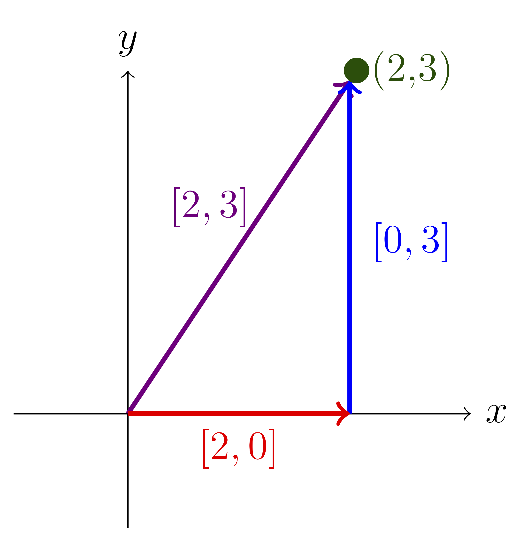
We can get from the origin to the point \((2,3)\) by walking east 2 blocks and north 3.
\begin{equation*}
2\left(\begin{array}{r}1 \\ 0 \end{array}\right)
+3\left(\begin{array}{r}0 \\ 1 \end{array}\right)
=\left(\begin{array}{r}2 \\ 3 \end{array}\right)
\end{equation*}
Figure 3.4.1. Path one with the elementary basis \(\mathcal{E}_2\text{.}\)
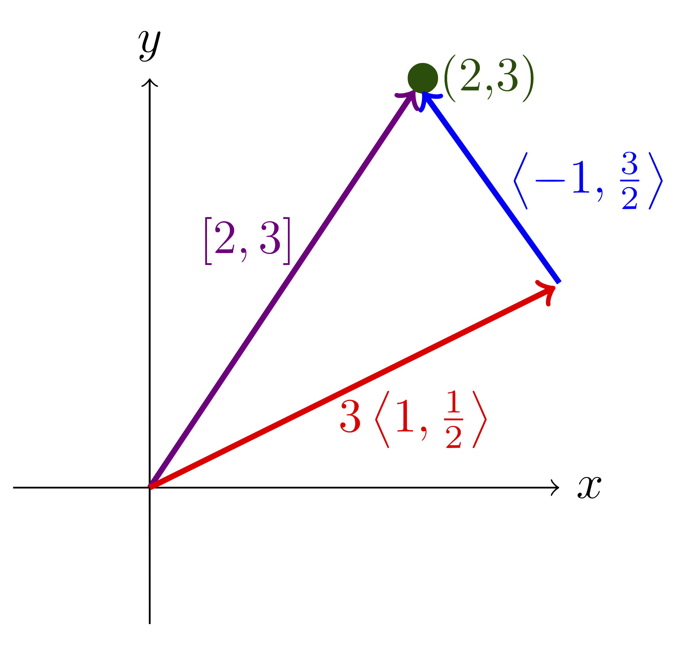
We can get there by walking northeast(ish) 3 blocks and northwest(ish) 1.
\begin{equation*}
3\left(\begin{array}{r}1 \\ 1/2 \end{array}\right)
+\left(\begin{array}{r}-1 \\ 3/2 \end{array}\right)
=\left(\begin{array}{r}2 \\ 3 \end{array}\right)
\end{equation*}
Figure 3.4.2. Path two with some basis \(\mathcal{B}\text{.}\)
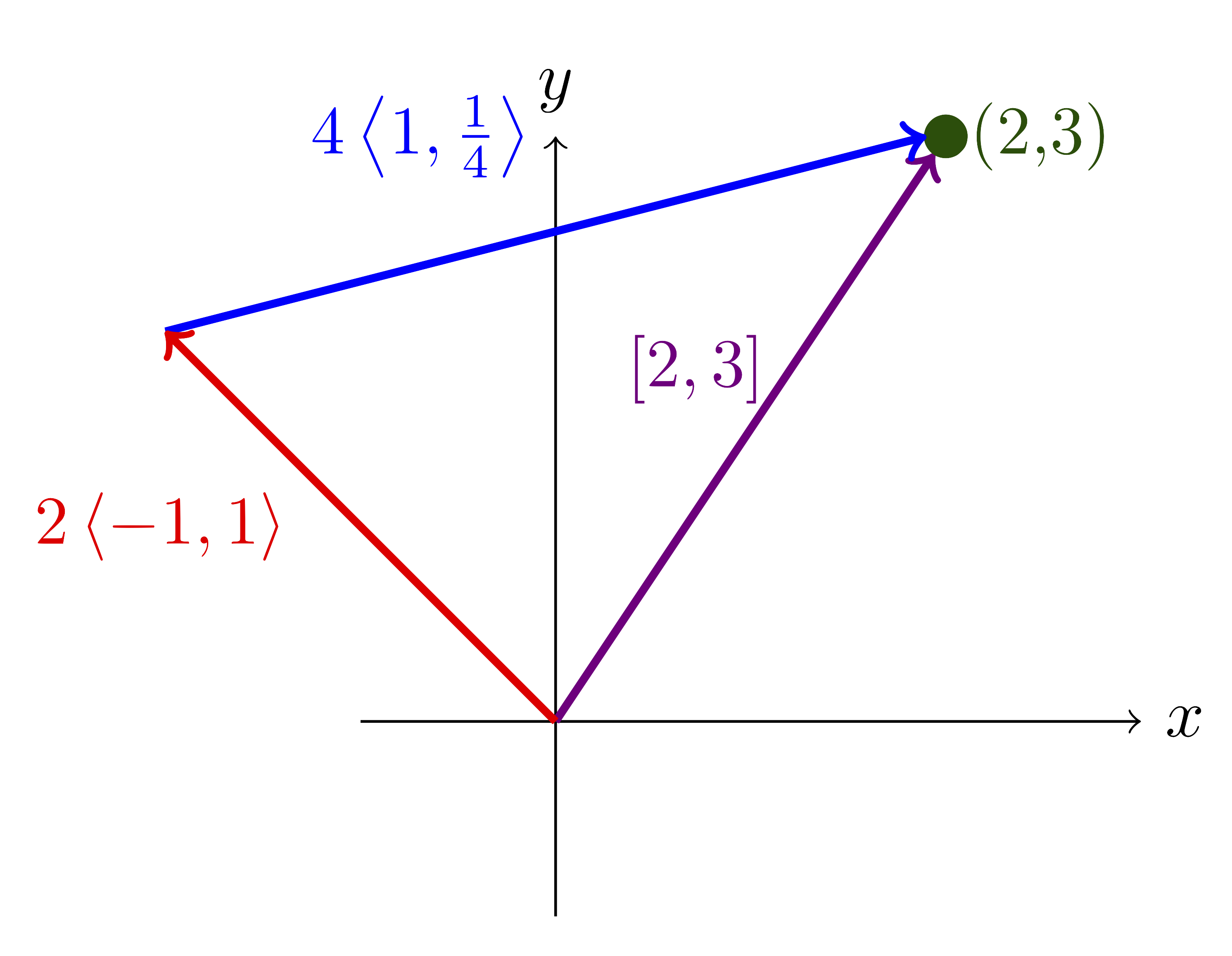
We can get there by walking northwest(ish) 2 blocks and northeast(ish) 4.
\begin{equation*}
2\left(\begin{array}{r}-1 \\ 1 \end{array}\right)
+4\left(\begin{array}{r}1 \\ 1/4 \end{array}\right)
=\left(\begin{array}{r}2 \\ 3 \end{array}\right)
\end{equation*}
Figure 3.4.3. Path three with some basis \(\mathcal{D}\text{.}\)
In each case you get to the same place but using different paths. That is because in each case we are using different bases or coordinate systems.
In Figure 3.4.1 we follow the vectors in the basis
\begin{equation*}
\mathcal{E}_2=
\left\{
\vec{e}_1=\left(\begin{array}{r}1 \\ 0 \end{array}\right),
\vec{e}_2=\left(\begin{array}{r}0 \\ 1 \end{array}\right)
\right\}.
\end{equation*}
We say that the \(\mathcal{E}_2\)-coordinates for \((2,3)\) are
\begin{equation*}
Rep_{\mathcal{E}_2}
\left(
\begin{array}{r}
2 \\ 3
\end{array}
\right)=
\left(
\begin{array}{r}
2 \\ 3
\end{array}
\right)
\end{equation*}
because
\begin{equation*}
2\left(\begin{array}{r}1 \\ 0 \end{array}\right)
+3\left(\begin{array}{r}0 \\ 1 \end{array}\right)
=\left(\begin{array}{r}2 \\ 3 \end{array}\right).
\end{equation*}
In Figure 3.4.2 we follow the vectors in the basis
\begin{equation*}
\mathcal{B}=
\left\{
\vec{\beta}_1=\left(\begin{array}{r}1 \\ 1/2 \end{array}\right),
\vec{\beta}_2=\left(\begin{array}{r}-1 \\ 3/2 \end{array}\right)
\right\}.
\end{equation*}
We say that the \(\mathcal{B}\)-coordinates for \((2,3)\) are
\begin{equation*}
Rep_{\mathcal{B}}
\left(
\begin{array}{r}
2 \\ 3
\end{array}
\right)=
\left(
\begin{array}{r}
3 \\ 1
\end{array}
\right)
\end{equation*}
because
\begin{equation*}
3\left(\begin{array}{r}1 \\ 1/2 \end{array}\right)
+1\left(\begin{array}{r}-1 \\ 3/2 \end{array}\right)
=\left(\begin{array}{r}2 \\ 3 \end{array}\right).
\end{equation*}
In Figure 3.4.3 we follow the vectors in the basis
\begin{equation*}
\mathcal{D}=
\left\{
\vec{\delta}_1=\left(\begin{array}{r}-1 \\ 1 \end{array}\right),
\vec{\delta}_2=\left(\begin{array}{r}1 \\ 1/4 \end{array}\right)
\right\}.
\end{equation*}
We say that the \(\mathcal{D}\)-coordinates for \((2,3)\) are
\begin{equation*}
Rep_{\mathcal{D}}
\left(
\begin{array}{r}
2 \\ 3
\end{array}
\right)=
\left(
\begin{array}{r}
2 \\ 4
\end{array}
\right)
\end{equation*}
because
\begin{equation*}
2\left(\begin{array}{r}-1 \\ 1 \end{array}\right)
+4\left(\begin{array}{r}1 \\ 1/4 \end{array}\right)
=\left(\begin{array}{r}2 \\ 3 \end{array}\right).
\end{equation*}
In each case the coordinates for the point \((2,3)\) are the coefficients for a linear combination of basis vectors.
Definition 3.4.4 . \(\mathcal{B}\)-Coordinates.
Given a basis
\begin{equation*}
\mathcal{B}=\left\{\vec{\beta}_1,\, \vec{\beta}_2,\, \ldots,\, \vec{\beta}_k\right\}
\end{equation*}
the \(\mathcal{B}\)-coordinates for a point or vector \(\vec{p}\) are the coefficients \(b_1,\, b_2,\, \ldots,\, b_k\) so that
\begin{equation*}
\vec{p}=b_1\vec{\beta}_1+b_2\vec{\beta}_2+\cdots+b_k\vec{\beta}_k
\end{equation*}
and we write
\begin{equation*}
Rep_{\mathcal{B}}(\vec{p})=
\left[
\begin{array}{l}
b_1\\ b_2\\ \vdots\\ b_k
\end{array}
\right].
\end{equation*}
Finally, we can connect this to matrices by observing that if the columns of a matrix are the basis vectors then when we multiply that by a representation we get our point, for example
\begin{equation*}
\left(\vec{\beta}_1\ \vec{\beta}_2\right)Rep_{\mathcal{B}}
\left(\begin{array}{r}2 \\ 3 \end{array}\right)
=
\left(
\begin{array}{rr}
1 \amp -1\\
1/2 \amp 3/2
\end{array}
\right)
\left(\begin{array}{r}3 \\ 1 \end{array}\right)
=
\left(\begin{array}{r}2 \\ 3 \end{array}\right).
\end{equation*}
Subsection 3.4.2 Changing Bases
Investigation 3.4.1 . \(\mathcal{B}\) to \(\mathcal{E}_2\).
The elementary or standard basis is
\begin{equation*}
\mathcal{E}_2=
\left\{
\vec{e}_1=\left(\begin{array}{r}1 \\ 0 \end{array}\right),
\vec{e}_2=\left(\begin{array}{r}0 \\ 1 \end{array}\right)
\right\}.
\end{equation*}
Let \(\mathcal{B}\) be the basis
\begin{equation*}
\mathcal{B}=
\left\{
\vec{\beta}_1=\left(\begin{array}{r}1 \\ 1/2 \end{array}\right),
\vec{\beta}_2=\left(\begin{array}{r}-1 \\ 3/2 \end{array}\right)
\right\}
\end{equation*}
as above. If we have a vector written in terms of \(\mathcal{B}\text{,}\)
\begin{equation*}
Rep_{\mathcal{B}}\left(\vec{v}\right)=
\left(
\begin{array}{r}
-1 \\ 3
\end{array}
\right)
\end{equation*}
and we want \(Rep_{\mathcal{E}_2}(\vec{v})\) then we multiply by the matrix
\begin{equation*}
Rep_{\mathcal{B},\mathcal{E}_2}=
\left(
\begin{array}{rr}
1 \amp -1 \\
1/2\amp 3/2
\end{array}
\right).
\end{equation*}
So we get,
\begin{align*}
Rep_{\mathcal{E}_2}(\vec{v})\amp = Rep_{\mathcal{B},\mathcal{E}_2}\, Rep_{\mathcal{B}}\left(\vec{v}\right)\\
\amp =
\left(
\begin{array}{rr}
1 \amp -1 \\
1/2\amp 3/2
\end{array}
\right)\,
\left(
\begin{array}{r}
-1 \\ 3
\end{array}
\right)\\
\amp =
\left(
\begin{array}{r}
-4 \\ 4
\end{array}
\right).
\end{align*}
To change from any basis
\begin{equation*}
\mathcal{B}=\left\{\vec{\beta}_1,\, \vec{\beta}_2,\, \ldots,\, \vec{\beta}_k\right\}
\end{equation*}
to \(\mathcal{E}_k\) multiply by the matrix
\begin{equation*}
Rep_{\mathcal{B},\mathcal{E}_k}=\left(\vec{\beta}_1\ \vec{\beta}_2\ \cdots\ \vec{\beta}_k\right)
\end{equation*}
each of whose columns is an element of \(\mathcal{B}\text{.}\)
Investigation 3.4.2 . \(\mathcal{E}_2\) to \(\mathcal{B}\).
Let \(\mathcal{E}_2\) and \(\mathcal{B}\) be the same as before and suppose
\begin{equation*}
Rep_{\mathcal{E}_2}(\vec{w})=
\left(
\begin{array}{r}
7\\-2
\end{array}
\right)
\end{equation*}
to change from \(\mathcal{E}_2\) to \(\mathcal{B}\) multiply by the matrix
\begin{equation*}
Rep_{\mathcal{E}_2,\mathcal{B}}=
\left(
\begin{array}{rr}
1 \amp -1 \\
1/2\amp 3/2
\end{array}
\right)^{-1}=
\left(
\begin{array}{rr}
3/4 \amp 1/2 \\
-1/4\amp 1/2
\end{array}
\right).
\end{equation*}
So we get,
\begin{align*}
Rep_{\mathcal{B}}(\vec{w})\amp = Rep_{\mathcal{E}_2,\mathcal{B}}\, Rep_{\mathcal{E}_2}\left(\vec{w}\right)\\
\amp =
\left(
\begin{array}{rr}
3/4 \amp 1/2 \\
-1/4\amp 1/2
\end{array}
\right)\,
\left(
\begin{array}{r}
7 \\ -2
\end{array}
\right)\\
\amp =
\left(
\begin{array}{r}
17/4 \\ -11/4
\end{array}
\right).
\end{align*}
To change from \(\mathcal{E}_k\) to any basis
\begin{equation*}
\mathcal{B}=\left\{\vec{\beta}_1,\, \vec{\beta}_2,\, \ldots,\, \vec{\beta}_k\right\}
\end{equation*}
multiply by the matrix
\begin{equation*}
Rep_{\mathcal{E}_k,\mathcal{B}}=(Rep_{\mathcal{B},\mathcal{E}_k})^{-1}=\left(\vec{\beta}_1\ \vec{\beta}_2\ \cdots\ \vec{\beta}_k\right)^{-1}.
\end{equation*}
Investigation 3.4.3 . \(\mathcal{B}\) to \(\mathcal{D}\).
Finally, let
\begin{equation*}
\mathcal{D}=
\left\{
\vec{\delta}_1=\left(\begin{array}{r}-1 \\ 1 \end{array}\right),
\vec{\delta}_2=\left(\begin{array}{r}1 \\ 1/4 \end{array}\right)
\right\}.
\end{equation*}
and let \(\mathcal{B}\) and \(\mathcal{E}_2\) be as before. Suppose also that
\begin{equation*}
Rep_{\mathcal{B}}\left(\vec{v}\right)=
\left(
\begin{array}{r}
-1 \\ 3
\end{array}
\right).
\end{equation*}
if we want to find \(Rep_{\mathcal{D}}(\vec{v})\) then multiply by the matrix
\begin{align*}
Rep_{\mathcal{B},\mathcal{D}}\amp=Rep_{\mathcal{E}_2,\mathcal{D}}Rep_{\mathcal{B},\mathcal{E}_2}\\
\amp=
\left(
\begin{array}{rr}
-1 \amp 1 \\
1\amp 1/4
\end{array}
\right)^{-1}
\left(
\begin{array}{rr}
1 \amp -1 \\
1/2\amp 3/2
\end{array}
\right)\\
\amp=
\left(
\begin{array}{rr}
-1/5 \amp 4/5 \\
4/5\amp 4/5
\end{array}
\right)
\left(
\begin{array}{rr}
1 \amp -1 \\
1/2\amp 3/2
\end{array}
\right)\\
\amp=
\left(
\begin{array}{rr}
1/5 \amp 7/5 \\
6/5\amp 2/5
\end{array}
\right).
\end{align*}
So that we get
\begin{equation*}
Rep_{\mathcal{D}}(\vec{v})=Rep_{\mathcal{B},\mathcal{D}}Rep_{\mathcal{B}}(\vec{v})=
\left(
\begin{array}{rr}
1/5 \amp 7/5 \\
6/5\amp 2/5
\end{array}
\right)
\left(
\begin{array}{r}
-1 \\ 3
\end{array}
\right)=
\left(
\begin{array}{r}
4 \\ 0
\end{array}
\right).
\end{equation*}
We can verify that this is correct because
\begin{equation*}
-1\vec{\beta}_1+3\vec{\beta}_2=
\left(
\begin{array}{r}
-4 \\ 4
\end{array}
\right)
\end{equation*}
and
\begin{equation*}
4\vec{\delta}_1+0\vec{\delta}_2=
\left(
\begin{array}{r}
-4 \\ 4
\end{array}
\right).
\end{equation*}
In general if
\begin{equation*}
\mathcal{B}=\left\{\vec{\beta}_1,\, \vec{\beta}_2,\, \ldots,\, \vec{\beta}_k\right\}
\end{equation*}
and
\begin{equation*}
\mathcal{D}=\left\{\vec{\delta}_1,\, \vec{\delta}_2,\, \ldots,\, \vec{\delta}_k\right\}
\end{equation*}
then
\begin{align*}
Rep_{\mathcal{B},\mathcal{D}}\amp=Rep_{\mathcal{E}_2,\mathcal{D}}Rep_{\mathcal{B},\mathcal{E}_2}\\
\amp=(Rep_{\mathcal{D},\mathcal{E}_2})^{-1}Rep_{\mathcal{B},\mathcal{E}_2}\\
\amp=\left(\vec{\delta}_1\ \vec{\delta}_2\ \cdots\ \vec{\delta}_k\right)^{-1}
\left(\vec{\beta}_1\ \vec{\beta}_2\ \cdots\ \vec{\beta}_k\right).
\end{align*}
Investigation 3.4.4 . Back to the Beginning.
We started above with
\begin{equation*}
Rep_{\mathcal{E}_2}
\left(
\begin{array}{r}
2 \\ 3
\end{array}
\right)=
\left(
\begin{array}{r}
2 \\ 3
\end{array}
\right),\
Rep_{\mathcal{B}}
\left(
\begin{array}{r}
2 \\ 3
\end{array}
\right)=
\left(
\begin{array}{r}
3 \\ 1
\end{array}
\right),\ \mbox{ and }
Rep_{\mathcal{D}}
\left(
\begin{array}{r}
2 \\ 3
\end{array}
\right)=
\left(
\begin{array}{r}
2 \\ 4
\end{array}
\right).
\end{equation*}
Now, we know that if we multiply the first one,
\begin{equation*}
Rep_{\mathcal{E}_2}\left(\begin{array}{r}2\\3\end{array}\right)=
\left(
\begin{array}{r}
2 \\ 3
\end{array}
\right)
\end{equation*}
by
\begin{equation*}
Rep_{\mathcal{E}_2,\mathcal{B}}=
\left(
\begin{array}{rr}
3/4 \amp 1/2 \\
-1/4\amp 1/2
\end{array}
\right)
\end{equation*}
or
\begin{equation*}
Rep_{\mathcal{E}_2,\mathcal{D}}=
\left(
\begin{array}{rr}
-1/5 \amp 4/5 \\
4/5\amp 4/5
\end{array}
\right)
\end{equation*}
we get the other two. That is we have a reliable, algorithmic way to change from one basis to another in the same dimension.
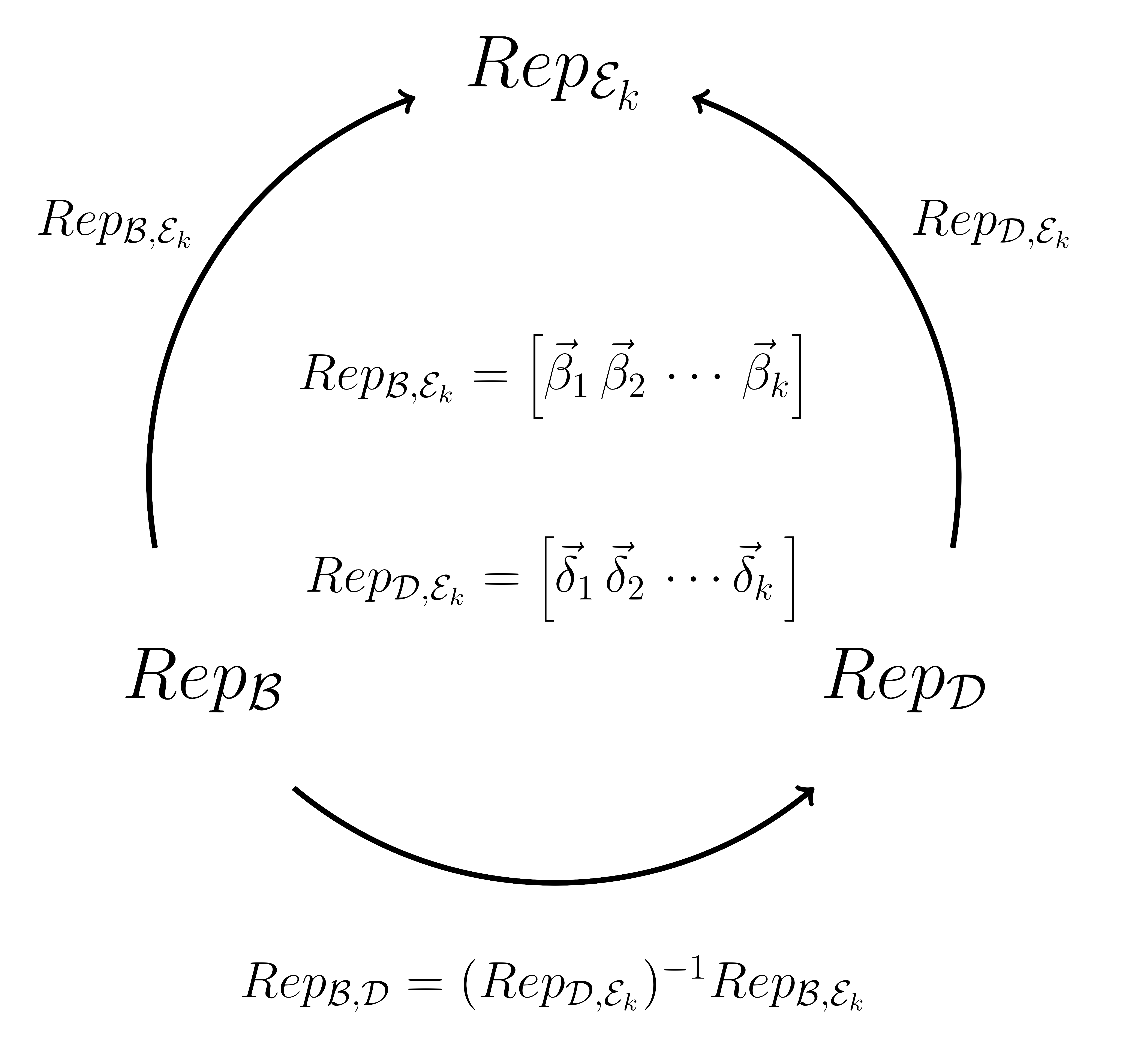
Summary Diagram for Bases Changes:
Figure 3.4.5. Changing from \(\mathcal{B}\) to other bases.
Subsection 3.4.3 Changing Morphisms
Investigation 3.4.5 . Change a transformation of \(\mathcal{E}_2\) to one from \(\mathcal{B}\) to \(\mathcal{D}\).
Let \(\mathcal{E}_2\) be as bove and let
\begin{equation*}
\mathcal{E}_3=
\left\{
\vec{e}_1=
\left(
\begin{array}{r}
1 \\ 0 \\0
\end{array}
\right),\, \vec{e}_2=
\left(
\begin{array}{r}
0 \\ 1 \\0
\end{array}
\right),\, \vec{e}_3=
\left(
\begin{array}{r}
0 \\ 0 \\1
\end{array}
\right)
\right\}
\end{equation*}
Define a transformation \(P\) from \(\mathbb{R}^3\) to \(\mathbb{R}^2\) by
\begin{equation*}
P(\vec{v})=(x,y).
\end{equation*}
From before the matrix for \(P\) is
\begin{equation*}
A=
\left(
\begin{array}{rrr}
1 \amp 0 \amp 0 \\
0 \amp 1 \amp 0
\end{array}
\right)
\end{equation*}
and it maps \(\mathcal{E}_3\) to \(\mathcal{E}_2\text{.}\)
Now suppose that we want the transformation to change vectors with coordinates in the basis
\begin{equation*}
\mathcal{B}=
\left\{
\vec{\beta}_1=\left(\begin{array}{r}1 \\ -2 \\ 0\end{array}\right),
\vec{\beta}_2=\left(\begin{array}{r}0 \\ 3 \\ 1 \end{array}\right)
\vec{\beta}_3=\left(\begin{array}{r}1 \\ 0 \\ 1 \end{array}\right)
\right\}
\end{equation*}
to vectors in terms of the basis
\begin{equation*}
\mathcal{D}=
\left\{
\vec{\delta}_1=\left(\begin{array}{r}-1 \\ 1 \end{array}\right),
\vec{\delta}_2=\left(\begin{array}{r}-3 \\ 4 \end{array}\right)
\right\}.
\end{equation*}
Do this by going from \(\mathcal{B}\) to \(\mathcal{E}_3\) to \(\mathcal{E}_2\) to \(\mathcal{D}\text{,}\)
\begin{align*}
(Rep_{\mathcal{D},\mathcal{E}_2})^{-1}\, A\, Rep_{\mathcal{B},\mathcal{E}_3} \amp =
\left(
\begin{array}{rr}
-4 \amp -3 \\
1 \amp 1\\
\end{array}
\right)
\left(
\begin{array}{rrr}
1 \amp 0 \amp 0 \\
0 \amp 1 \amp 0
\end{array}
\right)
\left(
\begin{array}{rrr}
1 \amp 0 \amp 1 \\
-2 \amp 3 \amp 0\\
0 \amp 1 \amp 1
\end{array}
\right)\\
\amp =
\left(
\begin{array}{rr}
-4 \amp -3 \\
1 \amp 1\\
\end{array}
\right)
\left(
\begin{array}{rrr}
1 \amp 0 \amp 1 \\
-2 \amp 3 \amp 0
\end{array}
\right)\\
\amp =
\left(
\begin{array}{rrr}
2 \amp -9 \amp -4 \\
-1 \amp 3 \amp 1
\end{array}
\right).
\end{align*}
Using this we get
\begin{equation*}
\left(
\begin{array}{r}
x \\ y \\ z
\end{array}
\right)\longmapsto
\left(
\begin{array}{r}
2x-9y-4z \\ -x+3y+z
\end{array}
\right).
\end{equation*}
Summary Diagram for Transformation Changes:
Figure 3.4.6. Changing transformations to new bases.